Mechanical vibration

Hints on the theory of mechanical vibrations. We intend to give here only an outline with the intention of framing the problem and providing the means to solve the simplest cases. Keep in mind that in almost all cases for a correct solution, the experience of a specialist is required.

Understanding various aspects of vibration theory enables one to choose the correct methods to reduce vibrations, for example by using various vibration dampers.

Therefore, for interventions of a certain amount of effort, we recommend consulting our guide on vibration:

VIBRATIONS

Vibration is defined as a quantity that oscillates around a reference value.

In the case of mechanical vibration, the oscillating quantity is a force or the displacement caused by it.

A mechanical vibration is characterized by:

• WIDTH, i.e., maximum variation in relation to the reference value.
• FREQUENCY, i.e., number of cycles (or oscillations) made in the unit of time (cycles/1″ or Hz).

The inverse of frequency is period.

Frequencies of practical interest in mechanical vibration range from fractions to a few hundred Hz.

Instead of amplitude, reference can be made to velocity or acceleration.

HARMONIC MOTION OF A MASS

Any mechanical system comprising an elastic element must be examined from an oscillatory point of view.

The simplest oscillatory system consists of a mass M and a spring of stiffness K (see Figure 1, oscillating system with one degree of freedom, without damping).

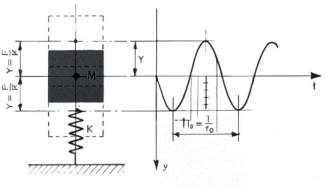
If a force F is applied to the mass M in this static system, displacing the mass’s center of gravity by a quantity Y, and the system is left free, it begins to vibrate with sinusoidal motion of constant amplitude and frequency f0.

The frequency thus determined is the eigenfrequency, that is, the frequency with which the system under consideration oscillates in the absence of external forces.

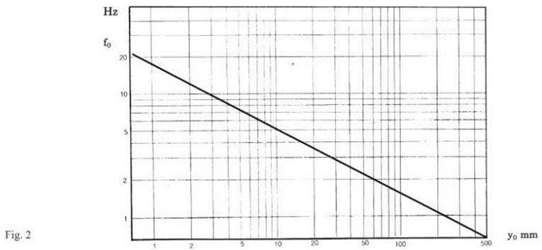
The formula is valid for any orientation in space. In the particular case of vertical oscillations we have:

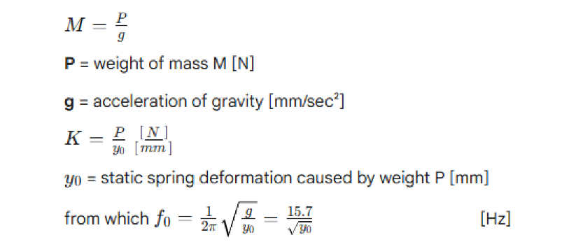
The trend of this equation is shown in Figure 2, where the eigenfrequency (fo) of a vertically oscillating system is directly determined as a function of the subsidence of the supports or the value of subtangent (y0).

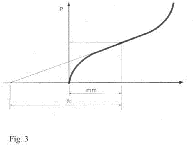
SUBTANGENT

(y0)

The actual yielding [mm] is not always equivalent to the value of the subtangent in elastic dowels.

In fact in metal springs, whose characteristic yielding loads are linear, the value of the subtangent is identified with the yielding of the spring.

In elastic supports it is an equivalent static yielding that is defined graphically as shown in Figure 3.

DAMPED OSCILLATIONS

In any real system, passive resistances must be taken into account.

Schematizing the passive resistances with a viscous-type damper, the system in Figure I yields the system in Figure 4.

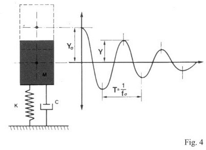
Viscous damping means that the resisting force Fr is proportional to the velocity of the motion:

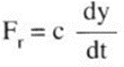
Where the coefficient of proportionality c is called the damping coefficient.

If Fr is expressed in [N], y in [mm] and t in [sec], c must be expressed in [N sec/mm].

Depending on the value of the damping coefficient c and the values of K and M, there are two types of motion:

aperiodic, i.e., with asymptotic return of the mass M to its original equilibrium position damped oscillating, i.e. with oscillations of the mass of progressively decreasing amplitude.

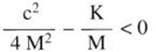
There is aperiodic motion when

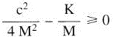
There is damped oscillatory motion when

The damping for which

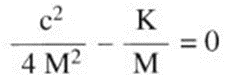
is defined as critical:

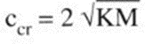
The units of measurement are those given above, namely: c is expressed in [N sec/mm], K in [N/mm], M in [N J sec2/mm].

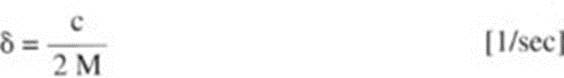
In most practical applications the motion is damped oscillating. In this case, the parameters characterizing the motion are:

damping modulus

logarithmic decrement

(Yn= amplitude of the nth oscillation)

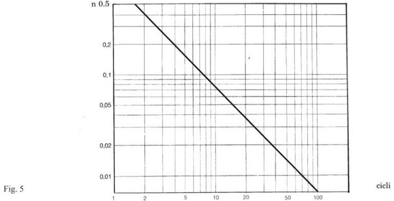
damping number or relative damping.

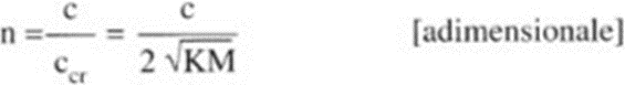
Fig. 5 shows the graph for the approximate determination of n based on the number of cycles required for the oscillation to stop:

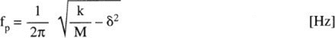
In the case of damped oscillations, the eigenfrequency of the system becomes

is often negligible. The error that is made by not considering it is equal to

The equation expressing the law of motion is:

y=y0e-δtcos(fpt+ϑ) [mm]

where

 t= time [sec]

 ωp= eigenpulse of the system (corresponding af fp) [rad/sec]

 y0= initial amplitude [mm]  = ϑinitial phase [rad]

FORCED OSCILLATIONS

If we superimpose a sinusoidal perturbing force F=P0 sin Ot on the previous system, where F and P0 are expressed in [N], with pulsation Ω in [rad], at steady state we will have:

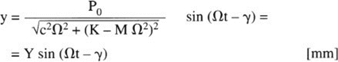
where the phase shift

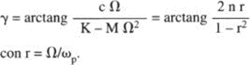
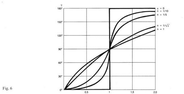
Note how the frequency of the forced oscillation is equal to that of the perturbing force regardless of the eigenfrequency of the system. In contrast, the phase shift γ depends on the characteristics of the system as well as the frequency of the perturbing force (see Fig. 6).

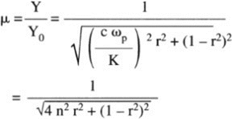
The ratio of the maximum strain Y that occurs as a result of the forced oscillation to the strain

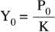
that would occur by statically applying the force P0 is called the resonance factor μ (Fig. 7)

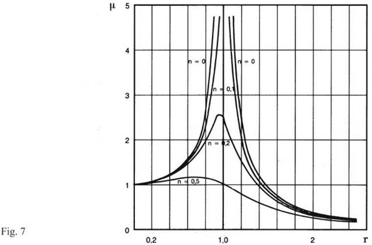
The maximum amplitude of the oscillation depends on the eigenfrequency of the system and the frequency of the perturbing force.

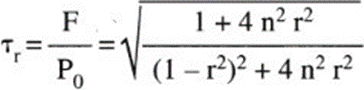
The ratio between the amplitude of the force F transmitted from the system to the structure and the perturbing force P0 is called the relative transmissibility coefficient τr, (fig. 8)

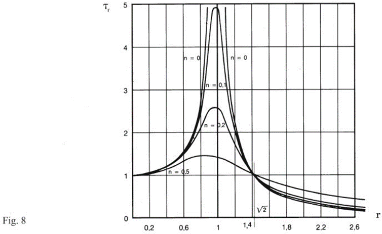
The difference between the resonance factor μ and the transmissibility coefficient τr should be well highlighted.

The former defines the amplitude of oscillation of the suspended mass; the latter indicates the isolation effect obtained.

It is evident from the trends in the graphs (Figures 7 and 8) that a high r=Ω/ωp ratio is favorable for both suspended mass oscillation and good isolation. It is recommended in applications to exceed r=2.

Conversely, high damping limits the oscillations of the suspended mass but causes a worsening in the isolation conditions.

For zero damping μ and τv coincide.

THE SHOCK

A shock is defined as a motion in which there is a sudden change in velocity.

Shock pulse is a perturbation characterized by a surge and subsequent decay of acceleration in a very short period of time.

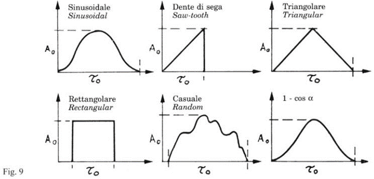
The shock pulse is usually defined by the peak amplitude A0 in g, the duration τ0 in milleseconds and the shape of the time- acceleration curve (see Figure 9).

Given the characteristics of the shock, we trace the acceleration G and displacement Y0 to which the elastic system is subjected by the formulas:

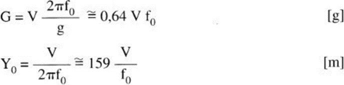
where

• f0 is the eigenfrequency of the system in Hz and V in m/sec measures the impact energy.
• V is obtained by integrating with respect to time the function acceleration o f the shock pulse.

In the absence of more precise guidance on the shape of the time-acceleration curve, it can be assumed:

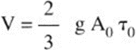
where

• A0= peak value of the acceleration in g;
• τ0= pulse duration in seconds.

Note how a low frequency decreases the magnitude of the transmitted force, but increases the deflection.

The above considerations apply to linear elastic (load- deflection) characteristics.

Note that for rubber this linearity is not verified and in addition there is another phenomenon that infirms t h e results, namely dynamic stiffening.

In the case of rubber, the calculations are therefore to be considered to be at fault.